
Understanding EUR/CHF Exchange Rate Breakpoints and Subperiods
This section presents an analysis of the Eur/chf exchange rate, focusing on identifying key breakpoints and the distinct subperiods they delineate. Our approach uses statistical methods to pinpoint shifts in exchange rate regimes, which are then cross-referenced with significant economic events to ensure logical consistency. A successful statistical model should accurately reflect known events, such as the Swiss National Bank’s (SNB) minimum exchange rate policy, by identifying its commencement and termination points.
Initially, numerous regression models were formulated, each designed to incorporate a maximum of one variable from each predefined category (e.g., only one stock index, one volatility index, etc.). This constraint is crucial to mitigate multicollinearity, a statistical issue arising from high correlations among variables within the same category. Subsequently, we estimated various sets of breakpoints, limiting both the maximum number of breakpoints and the minimum duration of the resulting subperiods. Given the potential for unreliable parameter estimations in very short subperiods, we established a minimum subperiod length of 20 months. Considering the timeline of economic events, we anticipated at least two breakpoints related to the SNB’s peg period and possibly another linked to the Global Financial Crisis. Consequently, our analysis primarily focused on models that identified up to three breakpoints. Table 1 summarizes the breakpoint estimates derived from 76 models that successfully detected three breakpoints, showing the frequency of detection for each breakpoint.
Table 1: Breakpoints Estimated (Minimum Subperiod: 20 Months, Maximum Breakpoints: Three)
| Breakpoint Estimate | Frequency |
|---|---|
| Mid-2007 | High |
| Late 2011 | Very High |
| Early 2015 | Very High |
The earliest breakpoint estimates tend to cluster around the onset of the global financial crisis, while the subsequent two breakpoints closely align with the initiation and conclusion of the SNB’s minimum exchange rate policy, often referred to as the “peg period.” By integrating these statistical findings with the timeline of economic events, we infer that the second and third breakpoints likely occurred around September 2011 and January 2015, respectively. Since our analysis uses monthly averages for the exchange rate, and the start and end of the peg period fall roughly in the middle of their respective months, we opted to exclude these months from the corresponding subperiods. This averaging effect might explain why our statistical methods identify breakpoints in adjacent months rather than precisely at the policy’s onset or conclusion.
For the initial breakpoint, our procedure identified three potential months in the latter half of 2007. To resolve this ambiguity, we utilized the overall (R^2) (for the entire sample period) achieved by selecting optimal variables for each subperiod based on our model. December 2007 was chosen as the first breakpoint, yielding an overall (adjusted) (R^2) of 31.41% (23.34%), which is superior to the alternatives of 30.10% (21.87%) for October 2007 and 30.13% (21.91%) for September 2007. Similar to our approach with the peg period breakpoints, we excluded December 2007 from the first two subsamples.
In summary, our breakpoint analysis segments the EUR/CHF exchange rate history into the following subperiods:
- January 2000–November 2007: Pre-financial crisis period.
- January 2008–August 2011: Financial crisis period leading up to the peg.
- October 2011–December 2014: SNB minimum exchange rate peg period.
- February 2015–December 2020: Post-peg period.
During the peg period, our analysis extends beyond the observed exchange rate to include a latent exchange rate calculated using option pricing theory, as developed by Hanke et al. (2019). This latent rate estimates where the EUR/CHF exchange rate would have been without the SNB’s intervention. Descriptive statistics for all variables across these subperiods are available in Table 9. Figure 3 illustrates rolling window correlations between all explanatory variables and the EUR/CHF exchange rate, using an 18-month window size.
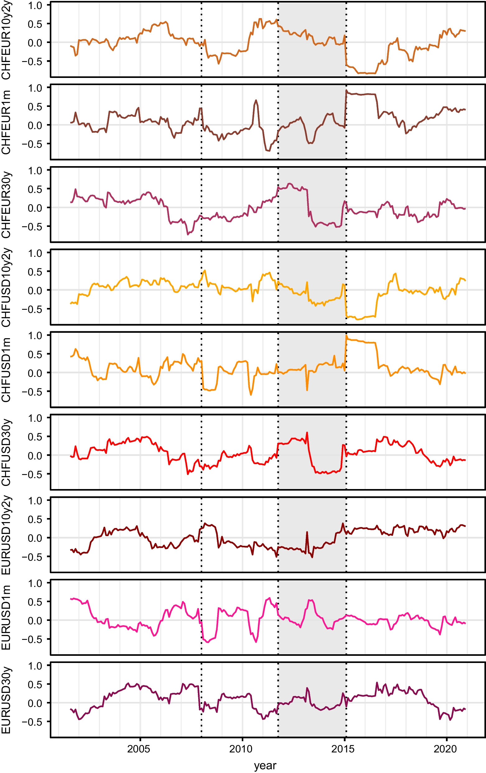 Rolling Window Correlations: Explanatory Variables vs. EUR/CHF Exchange Rate
Drivers of the EUR/CHF Exchange Rate Across Subperiods
For each subperiod identified through breakpoint analysis, we conducted regression analysis to determine the key drivers of the EUR/CHF exchange rate. Employing a step-forward approach, we iteratively selected the most significant drivers from a set of candidate variables, based on Newey-West adjusted p values. Given the potential for multicollinearity due to correlations among candidate drivers, we used Mallows’s (C_p) statistic as a criterion to prevent overfitting by limiting the number of variables. Additionally, the variance inflation factor (VIF) for each parameter was monitored to ensure multicollinearity was adequately controlled.
In the regression tables, all independent variables are standardized to have a zero mean and unit standard deviation. This standardization facilitates direct comparison of coefficient magnitudes, independent of the original variable scales. Each coefficient represents the change in the dependent variable (EUR/CHF exchange rate, multiplied by 100 for percentage representation) for a one-standard deviation increase in the corresponding driver.
We now detail the regression results for each identified subperiod, followed by a summary of the consistently selected variables and a comparison with driver selections from alternative variable selection methods, which serves as a robustness check for our findings.
Pre-Crisis Period Drivers (2000-2007)
The regression results for the pre-financial crisis period (January 2000–November 2007) are presented in Table 2. The DAX (German stock index) emerges as the primary driver. Model (1) shows that decreases in the DAX correlated with a strengthening of the Swiss franc against the euro during this period. This observation aligns with the Swiss franc’s established safe-haven status, where investors typically move funds into CHF during times of perceived risk in equity markets, as documented in prior research. The second variable selected by our step-forward procedure is the CHFUSD1m interest rate differential. Model (2) incorporates this, showing that among the CHF–EUR–USD interest rate differentials, CHFEUR differentials would intuitively have the most direct impact on EUR/CHF. While CHFEUR differentials are frequently selected in our broader analysis, the CHFUSD1m differential was prioritized for the pre-crisis period. This could be due to the substantial 53% correlation between CHFEUR1m and CHFUSD1m during this time, making the variable choice less distinct. The negative coefficient sign is consistent with expectations: higher Swiss franc interest rates relative to the US dollar (and by extension, the euro due to correlation) led to a stronger Swiss franc against the euro.
Table 2: Regression Results for the Pre-Crisis Period (January 2000–November 2007)
| Variable | Model (1) | Model (2) | Model (3) |
|---|---|---|---|
| DAX | -0.124** | -0.109** | -0.058 |
| CHFUSD1m | -0.071* | -0.072* | |
| SMI | -0.063 | ||
| Adjusted R-squared | 0.023 | 0.039 | 0.045 |
| Mallows’s Cp | 2.98 | 0.00 | 1.93 |
| VIF (DAX) | 1.00 | 1.03 | 2.01 |
| VIF (CHFUSD1m) | 1.03 | 1.04 | |
| VIF (SMI) | 1.98 |
Model (2) from Table 2 exhibits the lowest Mallows’s (C_p) statistic and is thus selected as the optimal model for this period. The SMI (Swiss Market Index) would have been the next variable to be included. However, column (3) illustrates why this model is deemed inferior based on Mallows’s (C_p). The high positive correlation between DAX and SMI during this era leads to SMI entering with a negative sign. The coefficient difference between DAX and SMI in model (3) approximates the DAX coefficient in model (2), while the VIFs for these two drivers are notably higher in model (3) compared to DAX in model (2). Despite an increase in adjusted (R^2), the corresponding rise in Mallows’s (C_p) from model (2) to model (3) indicates that the third variable should not be incorporated. It is worth noting that the explanatory power of the selected drivers is relatively low in the pre-crisis period, with an adjusted (R^2) of just 3.9% for the chosen model.
Financial Crisis Period Drivers (2008-2011)
During the financial crisis period (January 2008–August 2011), the slope difference between the Swiss franc and US dollar yield curves (CHFUSD10y2y) is identified as the most significant driver of the EUR/CHF exchange rate, as shown in Table 3. Adding the VSMI (Swiss Market Volatility Index) and the DAX further improves the model fit according to Mallows’s (C_p). Including additional variables, while increasing the adjusted (R^2), would worsen the (C_p) statistic, suggesting diminishing returns and potential overfitting.
Table 3: Regression Results for the Financial Crisis Period (January 2008–August 2011)
| Variable | Model (1) | Model (2) | Model (3) | Model (4) |
|---|---|---|---|---|
| CHFUSD10y2y | 0.398*** | 0.338*** | 0.288*** | 0.279*** |
| VSMI | 0.233*** | 0.299*** | 0.294*** | |
| DAX | -0.184** | -0.182** | ||
| CHFEUR10y2y | -0.038 | |||
| Adjusted R-squared | 0.143 | 0.200 | 0.232 | 0.233 |
| Mallows’s Cp | 3.93 | 0.00 | -1.87 | -1.74 |
| VIF (CHFUSD10y2y) | 1.00 | 1.14 | 1.25 | 1.57 |
| VIF (VSMI) | 1.14 | 1.49 | 1.51 | |
| VIF (DAX) | 1.28 | 1.28 | ||
| VIF (CHFEUR10y2y) | 1.44 |
A positive 10y2y spread in a country is generally seen as an indicator of favorable economic prospects, while a negative spread suggests potential economic downturn or recession. When comparing two currency areas, changes in the 10y2y spread differential can reflect shifts in their relative economic outlooks. Model (1) suggests that an increase in Switzerland’s 10y2y spread relative to the USD leads to a stronger Swiss franc against the euro. The subsequent variable selected, VSMI, acts as a crisis indicator. Equity volatility tends to be correlated across developed markets, with global economic uncertainty affecting all countries. The positive coefficient of VSMI is consistent with the Swiss franc’s safe-haven characteristics: increased equity volatility strengthens the Swiss franc. Model (3) includes the DAX as a further driver. Interestingly, the sign of the DAX coefficient flips to negative compared to the pre-crisis period, a phenomenon noted in prior literature indicating regime-dependent relationships between equity indices and EUR/CHF. The change in sign and magnitude of the VSMI coefficient between models (2) and (3) suggests an interaction effect between DAX and VSMI, likely due to their correlation. While including DAX is supported by the (C_p) statistic, incorporating CHFEUR10y2y is not, as shown in model (4). The compensatory effect between CHFUSD10y2y and CHFEUR10y2y becomes evident, and the increased VIF for CHFUSD10y2y confirms multicollinearity concerns. The drivers identified for the crisis period demonstrate markedly higher explanatory power, with an adjusted (R^2) of 20% for the selected model.
Peg Period Drivers (2011-2014)
Table 4 shows regression results for the SNB peg period (October 2011–December 2014). During this period, the short-term interest rate differential between the Swiss franc and the euro (CHFEUR1m) is the sole significant driver of the EUR/CHF exchange rate. Model (1) shows that, as expected, higher Swiss franc interest rates strengthen CHF against the euro. Adding the term structure slope difference (CHFEUR10y2y) in model (2) increases (R^2) but also raises Mallows’s (C_p). The positive sign of the CHFEUR10y2y coefficient is initially puzzling, but it is statistically insignificant and its inclusion affects the magnitude of the CHFEUR1m coefficient.
Table 4: Regression Results for the Peg Period (October 2011–December 2014)
| Variable | Model (1) | Model (2) | Model (3) | Model (4) |
|---|---|---|---|---|
| CHFEUR1m | 0.124** | 0.109** | 0.095 | 0.082 |
| CHFEUR10y2y | 0.057 | 0.053 | 0.051 | |
| VSMI | -0.042 | -0.043 | ||
| CHFEUR30y | 0.041 | |||
| Adjusted R-squared | 0.016 | 0.024 | 0.024 | 0.025 |
| Mallows’s Cp | 0.00 | 1.84 | 3.79 | 5.74 |
| VIF (CHFEUR1m) | 1.00 | 1.03 | 1.04 | 1.04 |
| VIF (CHFEUR10y2y) | 1.03 | 1.04 | 1.04 | |
| VIF (VSMI) | 1.00 | 1.00 | ||
| VIF (CHFEUR30y) | 1.00 |
Models (3) and (4) in Table 4 are included to illustrate the effects of alternative variable selection procedures that prioritize correlation over p values, which might select VSMI as an initial driver. Model (3) shows that starting with VSMI yields a better (R^2) than model (1) with CHFEUR1m, but VSMI’s coefficient is insignificant. CHFEUR1m would then be selected as the second driver, resulting in coefficients and p values similar to model (2). This comparison highlights the trade-off between variable selection methods: correlation-based methods often achieve higher (R^2) but may include insignificant coefficients.
Notably, foreign currency investments (FCI) are not selected as drivers during the peg period. This might be attributed to the SNB’s strong commitment to the 1.20 EUR/CHF floor, which reduced exchange rate variability, particularly during Q2-Q3 2012. SNB interventions, indicated by sharp increases in FCI, were prominent in Q3 2011 and Q2 2012. However, a significant influence of FCI on EUR/CHF is not statistically detected during the peg period.
The explanatory power of the selected driver (CHFEUR1m) during the peg period is very low, with an adjusted (R^2) of only 1.6%. This is likely due to the overriding influence of the SNB’s policy interventions. Table 5 presents regression results using the latent EUR/CHF exchange rate from Hanke et al. (2019) as the dependent variable during the peg period. For the latent rate, CHFEUR1m remains the primary driver, followed by the DAX. Including other interest rate differentials and term structure slopes improves (R^2) but is not recommended by Mallows’s (C_p). Model (2) shows expected signs for both variables: higher CHF interest rates strengthen CHF, and decreases in the DAX strengthen CHF against the euro, similar to the pre-crisis period. Comparing CHFEUR1m coefficients in Tables 4 and 5, the SNB’s peg policy significantly dampened the impact of short-term interest rate differentials on the observed EUR/CHF exchange rate.
Table 5: Regression Results for the Peg Period Using Latent Exchange Rate (October 2011–December 2014)
| Variable | Model (1) | Model (2) |
|---|---|---|
| CHFEUR1m | 0.249*** | 0.228*** |
| DAX | -0.112** | |
| Adjusted R-squared | 0.073 | 0.107 |
| Mallows’s Cp | 0.00 | -1.78 |
| VIF (CHFEUR1m) | 1.00 | 1.03 |
| VIF (DAX) | 1.03 |
Post-Peg Period Drivers (2015-2020)
The post-peg subperiod (February 2015–December 2020) exhibits the most diverse set of significant drivers for the EUR/CHF exchange rate. Notably, foreign currency investments (FCI) emerge as a significant driver in this subperiod, with very high statistical significance. A plausible explanation is that the SNB’s commitment to the 1.20 floor during the peg period required relatively moderate FCI to defend the rate. After abandoning the peg and ceasing explicit rate targets, the SNB likely needed to engage in more substantial FX market interventions, leading to a more than 50% increase in FCI post-peg. The positive coefficient for FCI is consistent with expectations: increased FCI weakens the Swiss franc.
Table 6: Regression Results for the Post-Peg Period (February 2015–December 2020)
| Variable | Model (1) | Model (2) | Model (3) | Model (4) | Model (5) |
|---|---|---|---|---|---|
| FCI | 0.409*** | 0.349*** | 0.313*** | 0.305*** | 0.305*** |
| SMI | 0.212*** | 0.186*** | 0.183*** | 0.182*** | |
| CHFEUR30y | -0.132** | -0.133** | -0.133** | ||
| EURUSD1m | -0.039 | -0.039 | |||
| CHFEUR1m | -0.002 | ||||
| Adjusted R-squared | 0.167 | 0.236 | 0.265 | 0.266 | 0.266 |
| Mallows’s Cp | 3.02 | 0.00 | -1.95 | 0.09 | 2.09 |
| VIF (FCI) | 1.00 | 1.06 | 1.11 | 1.12 | 1.12 |
| VIF (SMI) | 1.06 | 1.09 | 1.09 | 1.09 | |
| VIF (CHFEUR30y) | 1.04 | 1.04 | 1.04 | ||
| VIF (EURUSD1m) | 1.00 | 1.00 | |||
| VIF (CHFEUR1m) | 1.00 |
The SMI is the second variable selected, indicating that increases in the Swiss market index positively impact the Swiss franc, potentially due to portfolio-driven demand. Adding the long-term Swiss franc–euro interest rate differential (CHFEUR30y) further improves the model in column (3), with the expected negative sign. Including the EURUSD1m interest rate differential does not further reduce Mallows’s (C_p), and subsequent variables are insignificant, as seen in column (5). Model (3) is selected over model (4) for parsimony, among models with only significant coefficients. The adjusted (R^2) for model (3) is relatively high at 23.6%, and even model (1), with only FCI, achieves an adjusted (R^2) of 16.7%.
Summary of EUR/CHF Driver Regression Results
Table 7 summarizes the best regression models for the EUR/CHF exchange rate across each subperiod. Standardized coefficients allow for direct comparison of driver impacts within each period. The largest coefficient magnitudes are observed during the crisis and post-peg periods, which also exhibit the highest (R^2) values. The pre-crisis and peg periods show both lower driver impact and overall explanatory power.
Table 7: Summary of Best Regression Models for EUR/CHF Subperiods
| Variable | Pre-Crisis (2000-2007) | Crisis (2008-2011) | Peg (2011-2014) | Post-Peg (2015-2020) |
|---|---|---|---|---|
| DAX | -0.109** | -0.184** | ||
| CHFUSD1m | -0.071* | |||
| CHFUSD10y2y | 0.288*** | |||
| VSMI | 0.299*** | |||
| CHFEUR1m | 0.124** | |||
| FCI | 0.313*** | |||
| SMI | 0.186*** | |||
| CHFEUR30y | -0.132** | |||
| Adjusted R-squared | 0.039 | 0.232 | 0.016 | 0.265 |
Overall, the analysis reveals that different categories of drivers influence the EUR/CHF exchange rate, and their importance varies significantly across subperiods. In some instances, the impact of a driver even reverses sign between periods. These findings are consistent with prior research, which has documented time-varying correlations and sign changes for exchange rate drivers. Our descriptive approach identifies these shifts but does not delve into the underlying economic mechanisms that cause these variations. Explaining why a driver’s significance or impact changes across subperiods would require a different modeling approach, beyond the scope of this study.
Robustness Checks: REER Drivers and Alternative Selection Methods
To validate our methodology, we performed a robustness check by repeating the analysis using the Swiss real effective exchange rate (REER) as the dependent variable and comparing the resulting drivers to those found for the observed EUR/CHF exchange rate. The best models for the REER are presented in Table 10 in the Appendix. Table 8 compares the REER drivers to the EUR/CHF drivers for each subperiod, alongside drivers selected by alternative variable selection procedures.
Table 8: Driver Comparison by Subperiod and Selection Method
| Subperiod | EUR/CHF Drivers (p values) | REER Drivers (p values) | Alternative Methods Drivers |
|---|---|---|---|
| Pre-Crisis | DAX, CHFUSD1m | DAX, CHFEUR1m | (Varies) |
| Crisis | CHFUSD10y2y, VSMI, DAX | CHFUSD10y2y, VSMI, DAX | (Varies) |
| Peg | CHFEUR1m | CHFEUR1m | VSMI (often first) |
| Post-Peg | FCI, SMI, CHFEUR30y | FCI, SMI, CHFEUR30y | (Varies) |
Table 8 shows substantial overlap in the drivers selected for the REER and the observed EUR/CHF exchange rate, with approximately half of the drivers being identical. The sign reversals observed in beta coefficients between Tables 7 and 10 are due to the REER’s calculation and notation: CHF appreciation strengthens the REER, whereas EUR/CHF appreciation corresponds to a rate decrease.
Comparing our p-value based approach for EUR/CHF driver selection to alternative methods, we find broad agreement on the initial drivers across regimes, except for the peg period. The selection order is often consistent as well. The primary difference is that our approach results in more parsimonious models. In the peg period, some alternative methods prioritize VSMI as the primary or sole driver, while our method selects CHFEUR1m. The implications of these differing variable selections were discussed in detail in Section 4.2.3.